Artificial Neural Netoworks
CS123, Intro to AI
| Topics | |
|---|---|
| Overview of AI | Neural networks Deep learning |
| History of AI—Part 1 AI Problem Solving | Generative AI |
| Machine Learning—Part 1 Bayes' Rule | Prompt engineering |
| Machine Learning—Part 2 Regression and K-Nearest Neighbor | Custom chatbot creation |
| History of AI—Part 2 Midterm | Social and ethical issues of AI Final |
Table of Contents
Artificial Neural Networks (ANN)Neural Networks in the BrainPerceptronsMathematical ModelActivation FunctionLimitations of PerceptronsArtificial Neural NetworksDeep LearningCharacteristics of ANNsDiscussionElements of AI ExamplesBackpropagationBackpropagation in a PerceptronBackpropagation in an ANNConvolutional Neural Networks (CNN)History of CNN DevelopmentGenerative Adversarial Networks (GAN)ReferenceArticles and TutorialsInteractive Web Pages
Artificial Neural Networks (ANN)
Neural Networks in the Brain
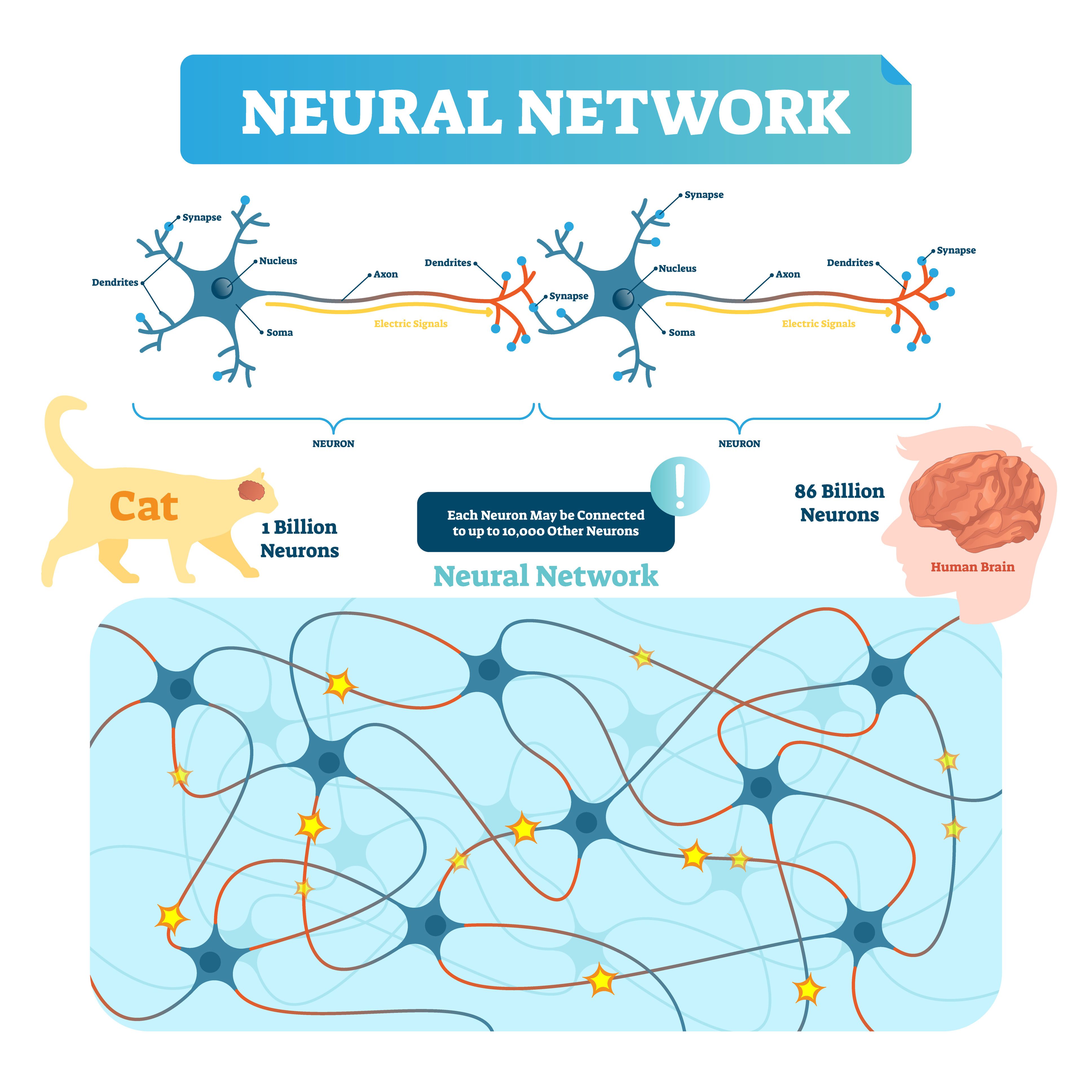
A biological neural network consists of interconnected neurons that communicate through axons, dendrites and synapses to process and transmit information. The dendrites are inputs to the neuron and the axon is the output of the neuron. The connection points are synapses. This intricate web of connections forms the basis for learning, memory, and behavior in living organisms.
Perceptrons
A perceptron is modeled on a single neuron.
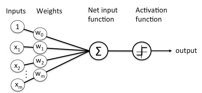
( ∑ is a the mathematical symbol for summation—aka addition.)
Mathematical Model
linear combination = intercept + weight1 × input1 + ... + weight6 × input6 (where ... is shorthand notation meaning that the sum include all the terms from 1 to 6).
The weights are used as multipliers on the inputs of the neuron, which are added up.
The intercept term is like the intercept in linear regression. This can be thought of as a fixed additional charge.
Activation Function
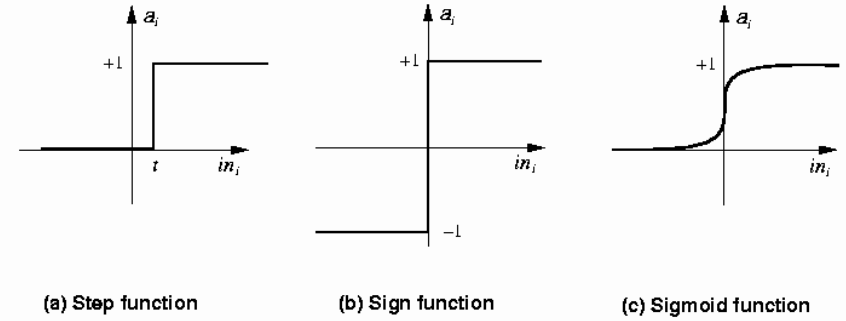
Once the linear combination has been computed, the neuron takes the linear combination and puts it through an activation function. Typical examples of the activation function include:
Step function: if the value of the linear combination is greater than zero, send a pulse (ON), otherwise do nothing (OFF)
Sign function: similar to the step function, but the output will be either +1 or -1.
Sigmoid (logistic) function: a “soft” version of the step function.
Limitations of Perceptrons
Perceptrons seemed to some, like Rosenblatt, the developer of the perceptron (1957,) to be the best way to advance the field of AI. But there were obstacles, which were publicized in detail by Minsky (who ironically developed the first neural network in 19511) and Pappert in their book Perceptrons (1969). These were two of the main obstacles:
Since there was only a single layer of nodes (neurons), they could only do linear classification (much like regression or Bayesian machine learning techniques).
There was no known way to write an algorithm for automatically learning the optimal weights for the connections.
Artificial Neural Networks
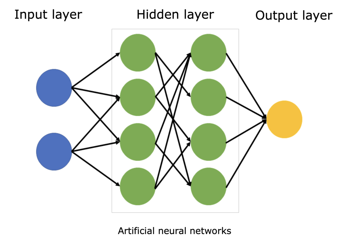
An artificial neural network (ANN) is a computational model inspired by the structure and function of neural networks in the brain. Each node, or "neuron", has multiple inputs, but one output. The nodes are arranged in layers and are interconnected. The input layer gets input data to be processed, the hidden layers do the processing and send data to an output layer (which could have more than one node.
Deep Learning
Techniques were developed to overcome some of the main the limitations identified by Minsky and Pappert.
Multiple Layers: The term “deep” refers to the use of multiple layers in the network—the hidden layers. These layers transform the input data into a more abstract and composite representation that goes beyond simple linear classification.
Self-learning: A number of algorithms were developed to set the weights on the connections in the ANN. One of these was Hebbian Learning, named after the psychologist Donald Hebb, it is based on a rule which states that if two neurons fire together, then the connection between them strengthens. This is often summarized as “Cells that fire together, wire together.”
Characteristics of ANNs
Information processing and storage (memory) are both done in the same place instead of memory and processing being separated.
Processing is done simultaneously (in parallel) across many neurons instead of sequentially.
Discussion
How is parallel processing in an ANN done?
Parallel processing in digital computers:
Time-slice
Multiple cores
Different types of processing units in consumer PCs:
CPU: typically 4 to 16 cores
GPU: NVIDIA GPUs can have hundreds or thousands of CUDA (Compute Unified Device Architecture) cores.
NPU: Typically have 10 to 20 cores.
Where is data in an ANN stored?
In a biological neural network, it is stored in the neurons
In an ANN it is ultimately stored in the computer's memory.
Elements of AI Examples
Discuss the X and O classifier
Discuss the happy or sad face classifier
There is an interactive classifier in E of AI and one made by your instructor.Does it make a difference whether faces are drawn so they fill the whole grid?
What if faces have different proportions?
Backpropagation
One of the main breakthroughs that led to progress on ANNs was the development of backpropagation in 1986 by Geoffrey Hinton, who is often referred to as the "godfather of AI".
Backpropagation, short for "backward propagation of errors," is an algorithm used to train ANNs by setting the weights on the connections.
Backpropagation in a Perceptron
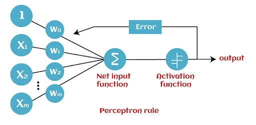
Backpropagation is a method used set the weights and improve accuracy. This is a summary of the steps:
Forward Pass: The perceptron processes training data to produce an output.
Error Calculation: The output is compared to the actual target to find the error.
Backward Pass: The error is used to adjust the weights, reducing the error.
This process repeats until the perceptron's predictions become accurate.
Backpropagation in an ANN
Here is a simplified summary of the steps in the algorithm:
Forward Propagation: Training data is passed through the network, from the input layer through the hidden layers to the output layer, to generate a prediction. This process is known as forward propagation.
Compute Loss (error): The prediction is compared with the actual target value to compute the loss (error). The loss function quantifies how far off the predictions are from the actual target values.
Backward Propagation: The loss is then propagated back through the network. This involves computing the gradient (slope) of the loss function with respect to the weights and biases in each layer of the network.
Update Weights and Biases: The weights and biases of the network are updated in the opposite direction to the gradient (in the opposite direction of the error). This is done to minimize the loss. The size of the update is determined by the learning rate, a hyperparameter that controls how fast the network learns.
Iterative Process: This process is repeated for many epochs (an epoch is one pass through the entire training dataset) until the network is adequately trained and the loss is minimized.
Convolutional Neural Networks (CNN)
When we tried to assign weights to an ANN that classified happy and sad faces, we discovered that the ANN had difficulty with:
Different sizes of faces
Faces that were positioned higher or lower in the input grid
Features (mouth size and position) that varied from face to face
CNNs resolves these problems and more using a convolution operation. This operation involves sliding a filter over the input data and performing element-wise multiplication followed by a sum. This process helps in extracting features from the input.
Here is a simplified description of the process (provided by MS Copilot):
Think of an image as a large field of different colored flowers. Now, suppose you want to identify patterns or features in this field, like areas of certain colors or color combinations.
The convolution operation is like using a small magnifying glass to look at one small area of the field at a time. This magnifying glass is what we call a "filter" or "kernel" in a Convolutional Neural Network (CNN).
As you move the magnifying glass across the field (or the image), you're focusing on one small area at a time. For each area, you're asking, "What's interesting here?" The answer could be "a lot of red flowers," "mostly blue flowers," "a mix of red and blue flowers," and so on. These are the "features" that the filter is learning to recognize.
The interesting thing is, you use the same magnifying glass (the same filter) to look at the entire field. This means you're looking for the same kind of features everywhere in the image. This is what gives CNNs their power: they can recognize the same features no matter where they appear in the image.
In summary, the convolution operation in a CNN is like using a magnifying glass to systematically scan across an image, looking for interesting features one small area at a time.
History of CNN Development
Convolutional Neural Networks (CNNs) were first developed and used in the 1980s. The foundational work was done by Kunihiko Fukushima and Yann LeCun.
Yann LeCun, in 1989, proposed a neural network architecture known as LeNet-5. This was the first successful implementation of a network that utilized the backpropagation algorithm for training, which is a standard method for training CNNs today. LeNet-5 was used for digit recognition tasks.
The significant breakthrough in the field of CNNs came in 2012 with the development of AlexNet by Alex Krizhevsky. AlexNet significantly outperformed previous image recognition algorithms and won the 2012 ImageNet contest with 85% accuracy.
Generative Adversarial Networks (GAN)
In this technique, two networks compete against each other. One of the networks is trained to generate images like the ones in the training data—it is called the generative network. The other network’s task is to evaluate images generated by the first network to see how well they correspond to real images from the training data – this one is called the adversarial network. These two combined then make up a generative adversarial network or a GAN.
Reference
Articles and Tutorials
What is a Perceptron: A Beginners Guide for Perceptron—Mayank Banoula, SimpliLearn, 2023.
Deep Learning—Ian Goodfellow, Yoshua Bengio, Aaron Courville, MIT Press, 2016
Neural Networks and Deep Learning—Michael A. Nielsen, Determination Press, 2015
Interactive Web Pages
Tensorflow Playground—Tinker with a neural network in your browser.
Understanding neural networks with TensorFlow Playground—Kaz Sato, Google Cloud, 2016.
Machine Learning Playground—Experiment with multiple ML models
GANPaint - Painting with Generative Models
Designed to Deceive: Do These People Look Real to You?—Kashmir Hill and Jeremy White, New York Times, Nov. 21, 2020.
In this interactive demo, notice that the slider features correspond to the features used when training the GAN.
 Intro to AI lecture notes by Brian Bird, written in 2024, revised in , are licensed under a Creative Commons Attribution-ShareAlike 4.0 International License.
Note: GPT-4 and GPT-4o were used to draft some parts of these notes.